« Impact of Amazon Prime in my purchase habits 09 Sep 2018
Summertime is always a great opportunity for me to read more frequently than usual. This August I’ve read two interesting books related to data analysis in python:
In Personal Finance with Python: using pandas, Requests and Recurrent last chapter, the author talked about times series forecasting and how he used Prophet to estimate his future expenses in Amazon.
The book referenced a CSV file including the author’s Amazon purchases since 2012, hence I guessed there might be a simple way to download a CSV report from Amazon including every purchase the logged in user did in the website. As I’ll explain in the following paragraphs I was wrong and it wasn’t that easy, but in any case that chapter gave me a hint to explore something I was curious about: What was the impact of becoming an Amazon Prime customer in my Amazon purchases habits?
No matter if you’re working with big or little data, the major steps you need to follow for data analysis can be summarized as follows (if you’re a data analyst and don’t agree with these steps, you’re probably right!):
- Data gathering: this step focuses on obtaining the data from one (in case you’re lucky) or more (the real world) sources.
- Data normalization: in case you have more than one source of data or data structure, a normalization phase is required (or at least recommended!).
- Data munging: “The difference between data found in many tutorials and data in the real world is that real-world data is rarely clean and homogeneous”. Great sentence by Jake VanderPlas in Python Data Science Handbook. He is right :-)
- Data analysis and plot: execute the right algorithm and plot the data in a graph that will help you to understand the meaning of the data (extract information out of the data).
In order to analyse the impact of Amazon Prime, I went through these four steps, which I’ll describe in the following paragraphs.
Data gathering
I googled “Amazon purchases CSV report” and apparently https://www.amazon.es/gp/b2b/reports was the place I was looking for (mind the .es domain).
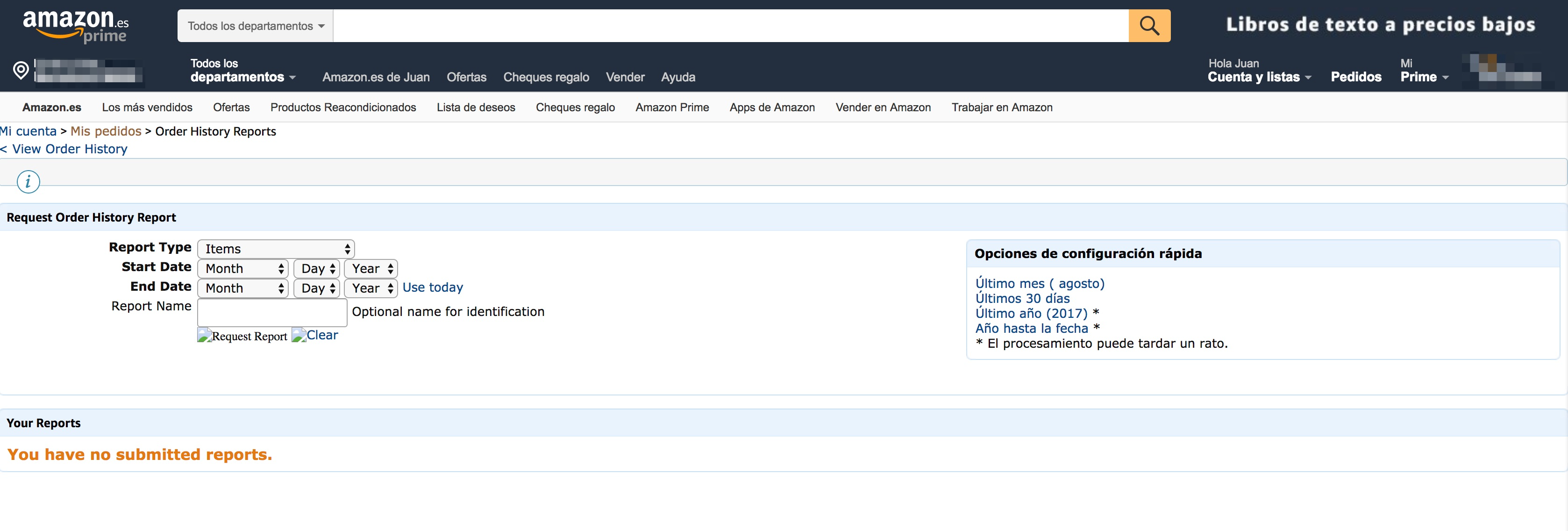
Well… a web form not using a single language is not what you’d expect from a trillion dollar valuation company.
I filled in the form to download the data and… uppss!! It didn’t work. So I went to the amazon.com site (instead of amazon.es), as I assumed there was a temporal issue in the Spain web portal. In amazon.com things indeed got better, now I had a web form with a single language (English) and I was able to download my CSV report.
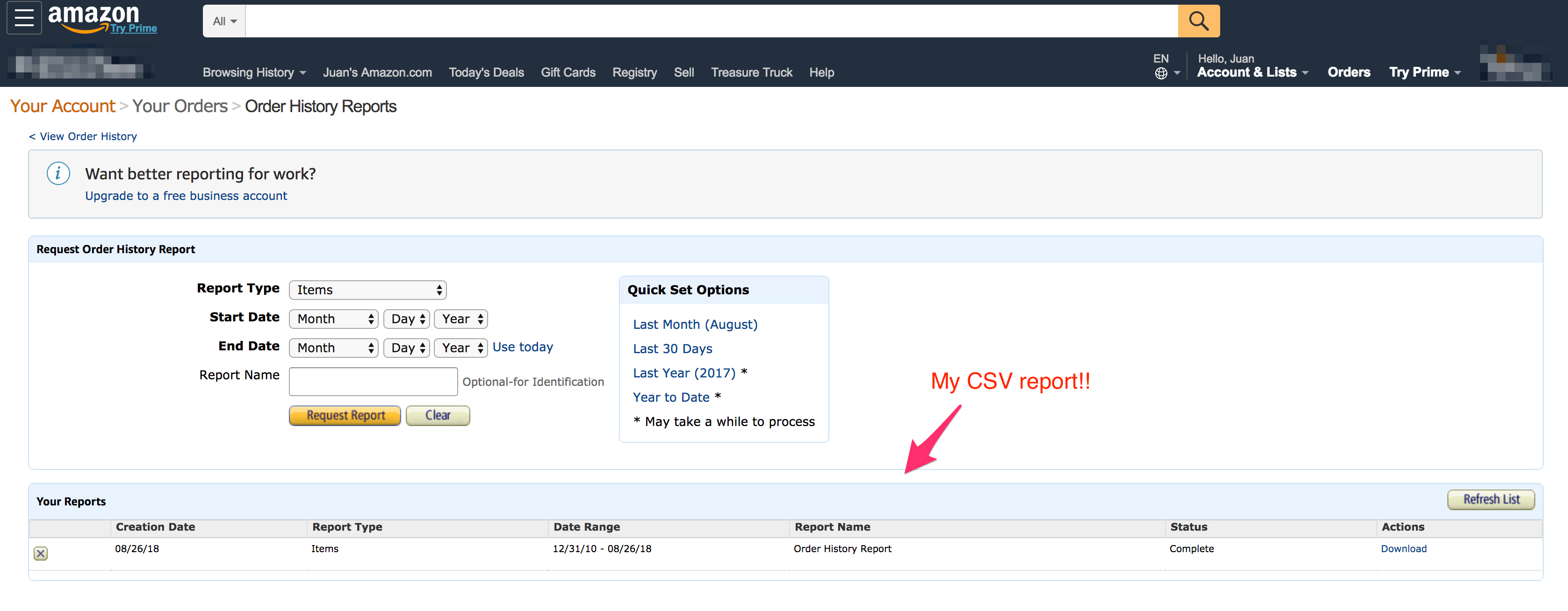
Wait!! The report included data only from 2011 to 2012. I was certainly sure I had purchased more stuff in Amazon in the following years, so something was wrong there.
Suddendly I realized it was some years ago when Amazon launched amazon.es website, and since then I was not able to buy anymore in amazon.com (at least if the same stuff was available in amazon.es). Apparently single sign on works like a charm between amazon.com and amazon.es, but each data report is available only in the website where the purchase was done, and after 2012 all my purchases had happened in amazon.es. Building global products is hard!!
I was able to review in Amazon Spain website the purchases I did since 2012, but as mentioned at the beginning I was not able to download an automatically generated report.
I decided to generate the CSV report manually. I’m not a really big Amazon customer so eventually it didn’t take me more than one hour to generate it.
Now I was ready for the first interesting step.
Data normalization
Cool, so now I had two files, juan-amazon-us.csv and juan-amazon-es.csv, each of them holding a report with my purchases in a single Amazon online store.
Next step was data normalization. I was specifically interested in:
- filter out fields from the CSV that I considered private data, so I could upload to the wild Internet the CSV report (in case someone is interested in playing with the Jupyter notebook).
- currency normalization: US items were purchased in dollars, while ES items were in euros. I decided to convert euros to dollars.
- merge both files: generate a single source for loading and analysing the data.
While python and a library like pandas might be a good fit
for tackling the topics above, I preferred to implement this step directly as an script on top of bash.
I have spent a considerable amount of time during my last year in the bash console,
so I felt pretty confident about it.
I did a couple of tests with the usual bash commands (cat, cut, awk, …) but eventually
I decided to give a try to jqlite.
jqlite is a wrapper on top of sqlite implemented by my colleague
@drslump, which provides a SQL interface on top of
tabular data (CSV, TSV, JSON).
It looked like a perfect match for the scenario I was interested in:
- SELECT for fetching those fields I was ok to expose, and filtering out those I was not.
- CASE…END for currency conversion.
- UNION ALL for merging both files.
I came up with the following query:
echo "SELECT date
      , orderId
      , CASE WHEN currency = \"€\" THEN amount*1.1 ELSE amount END as amount
     FROM (
         SELECT \"Order Date\" as date,
                \"Order ID\" as orderId,
                substr(\"Item Total\", 2) as amount,
                substr(\"Item Total\", 1,1) as currency
         FROM (
            SELECT * FROM SPAIN UNION ALL SELECT * FROM USA
         )
     )" \
| jqlite "data/juan-amazon-es.csv@SPAIN" "data/juan-amazon-us.csv@USA"
At this point, my data was filtered, normalized and combined in a single file, ready to move to the python and pandas world.
Data munging
With unnecessary fields dropped out and data normalisation done in the previous step, now it was time to model the data to be able to plot it with ease.
Pandas is a really convenient library for working with time series, and I really enjoyed learning about it with Python Data Science Handbook.
The steps I followed to model the data were:
- Load the CSV into memory and create a Panda DataFrame with the columns (date,orderId,amount).
- Reduce purchase time granularity from day to month.
- Set the month column as Pandas DataFrame index.
- Generate a Pandas Series having as index a time series from the minimum month when I made a purchase till now, and zeros as value.
- Calculate the number of purchases and total amount per month.
- Calculate the accumulated spent in every month.
- Fill NaN values with the relevant data.
You can find the actual code in the github repository that contains the Jupyter notebook.
Data analysis and plot
I became an Amazon prime customer in June 2017. In the following graphs you can see:
- the total amount spent from 2011 till 2018.
- the number of orders, per month.
Vertical line shows the exact moment when I became an Amazon Prime user.
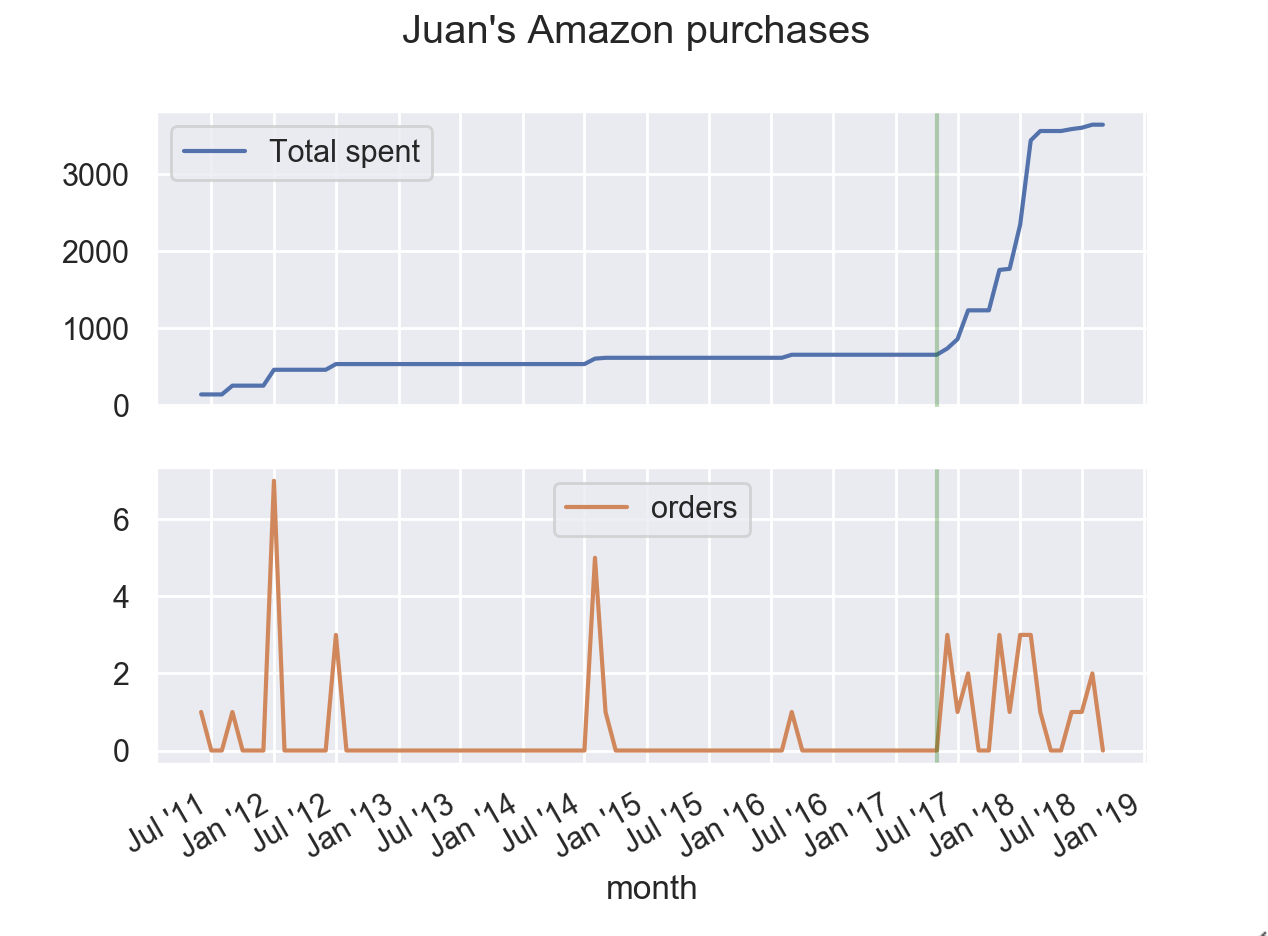
Conclusions
Even though the total amount spent grew considerable after me becoming an Amazon Prime customer, I think the most relevant conclusion is that after that date (June 2017) I’ve purchased in Amazon at least one item at almost every month.
So even though Amazon Prime price in Spain is
(was) cheap, it seems like a big win for Amazon to subsidize it.
Last, but not least, I’ll put some effort in reducing the amount of purchases I do in Amazon in favor of local shops.
« Home